CPU Usage During Simulation

Simulation Computation Threads

Time-series data is computed on a single thread (using only one CPU core at a time); other data can be computed in parallel.

Geometry Removal

Geometry removal is single-threaded because sequential cutting is required to obtain the correct CWE (Cutter-Workpiece Engagement). The workpiece geometry surface after removal appears in light pink, which typically indicates that the physics for that region have not yet been computed.

Physics Computation

Cutting force computation begins after CWE is obtained. Since it is independent of computation order, it runs in multi-threaded mode under normal conditions. Torque and other physical quantities are also computed in parallel during this stage.

Temperature computation must follow time-series order, so it converges back to a single thread.

The entire machining simulation alternates between these modes. Once a step is fully computed, it is colored according to the designated indicator.

Two Independent Cost Drivers

Total simulation time comes from two largely independent parts:

Per-step physics (force, torque, power, temperature, wear) — computed once per step. The total physics cost scales with the number of steps, which is set by the machining motion resolution together with the spindle revolutions along the toolpath. It does not depend on the mesh resolution, and it does not depend on the overall workpiece size.
Geometry removal (voxel subtraction) — its cost is set by the mesh resolution (MachiningResolution_mm). A finer mesh (smaller value) is more expensive; a coarser mesh (larger value) is cheaper. Removal work is localized to the tool–workpiece contact region, so it is roughly area-scaled and, again, largely independent of the bulk workpiece size.

MachiningResolution_mm genuinely controls the removal resolution — it is not clamped away or ignored. But because removal and physics run concurrently, the larger of the two costs governs wall-clock time:

When geometry removal dominates — the common case at the fine resolutions real NC machining needs — a finer mesh is much slower, and a coarser mesh reduces total time.
When the mesh is coarse enough that geometry removal is already cheap, several fixed per-step costs (physics, thermal/wear, per-step bookkeeping) dominate instead. Coarsening further — e.g. raising MachiningResolution_mm from 1.0 to 2.0 mm — then barely changes total time; to speed up, reduce the number of steps with a coarser motion resolution. (Note: 1–2 mm is already very coarse for NC machining.)

CPU Usage

Coarse Mesh — Physics-Bound

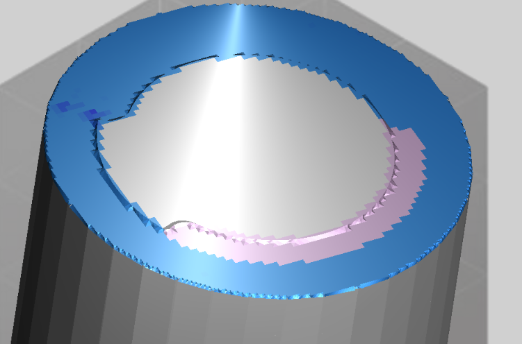
When the mesh is coarse (a large MachiningResolution_mm), geometry removal is faster than physics computation, so a large area of light pink follows behind the tool during simulation. There is a cap on the number of unfinished steps; geometry removal only proceeds when the count is within that limit. When physics computation cannot keep up with geometry removal, the number of pink steps stays constant.

In this scenario, the workload is primarily multi-core (physics computation), and you are more likely to see high multi-core CPU utilization. Making the mesh even coarser will not reduce total time — the step count (physics) is the limit.

Coarse mesh: geometry removal outruns physics, leaving a large pink trail

Fine Mesh — Geometry-Bound

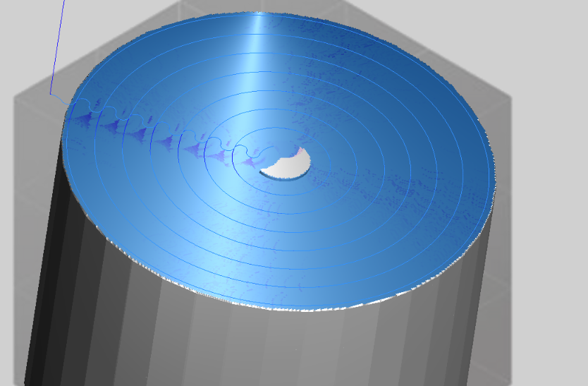
When the mesh is fine (a small MachiningResolution_mm), geometry removal is slower than physics computation, so the light pink area is barely visible.

In this scenario, the workload is primarily single-core (geometry computation), and a coarser mesh will reduce total time.

Fine mesh: physics keeps up with geometry removal, almost no pink trail

Balanced State

If the geometry resolution is such that geometry and physics computation do not bottleneck each other, the light pink area appears and fluctuates within a certain range. In this case, physics computation does not hold back geometry computation, and geometry computation is typically the performance bottleneck.

Optimization — One Burst, Then One Core

An NC optimization is not the play loop, and its CPU trace has a different shape. Exactly one of its stages is parallel: the per-step feed solve, which spreads the played steps across a private pool of workers running at below-normal thread priority, so it stays behind interactive work on the same machine. Every stage announced after it — the two feed constraints, the compensation build, the NC regeneration and the file write — runs on a single thread.

So an optimization shows one multi-core burst and then a single-core tail. A CPU sitting near one core's worth of load for the rest of the run is the expected shape, not a stalled run.

The host setting HiNC:OptCoreNum sizes that one parallel stage. The shipped value 0 gives it one worker per logical processor; any other value caps it at that many workers, which leaves more of the machine for other work and lengthens the burst. It changes nothing else: not the single-threaded stages that follow, and not the simulation loop above.

CPU Not Fully Utilized

Possible reasons why the CPU is not fully utilized include:

The operating system reserves headroom to ensure the GUI remains responsive. For example, Windows desktop applications (such as WPF) lower the priority of non-GUI threads by one level.
The software/hardware throughput has reached its limit for the process. The reported CPU usage may not reach 100%, but other resources such as cache and bus bandwidth may be saturated. System-level factors like branch misprediction are also not reflected in the reported CPU usage.

There is no setting that changes either of these. A CPU that looks idle during an NC optimization is a different question, and it is answered by the stage shape above rather than by this list.

Table of Contents